The KXY Data Valuation Function Works (Regression)
We consider 4 multi-dimensional toy regression problems where the latent function is known.
We show that the data valuation analysis of the kxy package is able to recover the true highest achievable performances (e.g. \(R^2\), RMSE, etc.) almost perfectly.
In [1]:
%load_ext autoreload
%autoreload 2

import pylab as plt
import pandas as pd
import numpy as np
np.random.seed(0)
import kxy
The Data
We use generative models of the form
We use the functional forms
with \(x_i \sim U\left([0, 1] \right)\) i.i.d. standard uniform, and \(\epsilon\) a Gaussian noise.
Background
The classic definitions of the \(R^2\) and the RMSE of a regression model \(y = f\left(\mathbf{x}\right) + \epsilon\) are respectively
and
These definitions are OK when \(y\) and \(\epsilon\) are Gaussian, but the variance terms fail to fully capture uncertainty in non-Gaussian distribution (e.g. fat-tails).
Note that, when \(y\) and \(\epsilon\) are Gaussian, we also have \(R^2\left(f\right) = 1- e^{-2I\left(y; f(\mathbf{x}) \right)}\) and \(\text{RMSE}\left(f\right) := \text{Var}(y) e^{-2I\left(y; f(\mathbf{x}) \right)}.\)
Given that entropies are better measures of uncertainty than the variance, we can use these formulae to define generalized versions of the \(R^2\) and the RMSE.
The theoretical best values these generalized versions may take (across all possible models) are easily found to be \(\bar{R}^2 = 1- e^{-2I\left(y;\mathbf{x}\right)}\) and \(\bar{RMSE} = \text{Var}(y) e^{-2I\left(y; \mathbf{x} \right)}.\)
Ground Truth Calculation
In this notebook, we choose various functional form for \(f_i\) and we choose a Gaussian residual \(\epsilon\). As such, we know the theoretical best values the classic \(R^2\) and RMSE may take.
However, we cannot calculate the true mutual information in closed form for all \(f_i\) but \(f_1\). Instead, we use as proxy for the best generalized \(R^2\) and RMSE achievable (for \(i>1\)) the best classic \(R^2\) and RMSE achievable.
This means that any deviation between our estimated highest generalized \(R^2\) (resp. lowest generalized RMSE) and the true highest classic \(R^2\) (resp. lowest classic RMSE) is a mix of estimation error and the fact that \(f_i(\mathbf{x})\) is non-Gaussian for \(i>1\).
Noise Variance
We consider various highest achievable classic \(R^2\) values (\(1., 0.99, 0.5, 0.25\)) and we infer the corresponding noise variance as \(\sigma^2 = \frac{1}{R^2}-1 = \text{RMSE}^2\).
In [2]:
# Sample size
n = 20000
d = 10
u = np.random.rand(n, d)
x = np.dot(u, 1./np.arange(1., d+1.))
x = 2.*x/(x.max()-x.min())
x = x-x.min()-1.

# Noiseless functions
names = [r'''$f_i(\mathbf{x}) \propto \sum_{i=1}^d\frac{x_i}{i}$''', \
         r'''$f_i(\mathbf{x}) \propto \sqrt{\left\vert \sum_{i=1}^d\frac{x_i}{i} \right\vert}$''', \
         r'''$f_i(\mathbf{x}) \propto -\left(\sum_{i=1}^d\frac{x_i}{i}\right)^3$''', \
         r'''$f_i(\mathbf{x}) \propto \tanh\left(\frac{5}{2}\sum_{i=1}^d\frac{x_i}{i}\right)$''']
fs = [lambda u: u, lambda u: -np.sqrt(np.abs(u)), lambda u: (-u)**3, lambda u: np.tanh(2.5*u)]

# Noise configurations
rsqs = np.array([1., .99, .75, .50, .25]) # Desired  Exact R^2
err_var = 1./rsqs-1.
err_std = np.sqrt(err_var) # Implied Exact RMSE assuming

# Generate the data
data = [[]]*len(rsqs)
for i in range(len(rsqs)):
    dfl = []
    for j in range(len(fs)):
        y_ = fs[j](x)
        y = y_/y_.std()
        y = y + err_std[i]*np.random.randn(x.shape[0])
        z = np.concatenate([y[:, None], u], axis=1)
        df = pd.DataFrame(z.copy(), columns=['y'] + ['x_%s' % i for i in range(d)])
        dfl += [df.copy()]

    data[i] = dfl
Data Valuation
In [3]:
estimated_rsqs = [[None for j in range(len(fs))] for i in range(len(rsqs))]
estimated_rmses = [[None for j in range(len(fs))] for i in range(len(rsqs))]

for i in range(len(rsqs)):
    print('\n\n')
    print(r'''-------------------------------------''')
    print(r'''Exact $R^2$: %.2f, Exact RMSE: %.2f''' % (rsqs[i], err_std[i]))
    print(r'''-------------------------------------''')
    for j in range(len(fs)):
        print()
        print('KxY estimation for %s' % names[j])
        dv = data[i][j].kxy.data_valuation('y', problem_type='regression')
        estimated_rsqs[i][j] = float(dv['Achievable R-Squared'][0])
        estimated_rmses[i][j] = float(dv['Achievable RMSE'][0])
        print(dv)
-------------------------------------
Exact $R^2$: 1.00, Exact RMSE: 0.00
-------------------------------------

KxY estimation for $f_i(\mathbf{x}) \propto \sum_{i=1}^d\frac{x_i}{i}$
[====================================================================================================] 100% ETA: 0s
  Achievable R-Squared Achievable Log-Likelihood Per Sample Achievable RMSE
0                 1.00                                 2.54        1.92e-02

KxY estimation for $f_i(\mathbf{x}) \propto \sqrt{\left\vert \sum_{i=1}^d\frac{x_i}{i} \right\vert}$
[====================================================================================================] 100% ETA: 0s
  Achievable R-Squared Achievable Log-Likelihood Per Sample Achievable RMSE
0                 1.00                                 2.50        2.01e-02

KxY estimation for $f_i(\mathbf{x}) \propto -\left(\sum_{i=1}^d\frac{x_i}{i}\right)^3$
[====================================================================================================] 100% ETA: 0s
  Achievable R-Squared Achievable Log-Likelihood Per Sample Achievable RMSE
0                 1.00                                 3.71        1.26e-02

KxY estimation for $f_i(\mathbf{x}) \propto \tanh\left(\frac{5}{2}\sum_{i=1}^d\frac{x_i}{i}\right)$
[====================================================================================================] 100% ETA: 0s
  Achievable R-Squared Achievable Log-Likelihood Per Sample Achievable RMSE
0                 1.00                                 3.09        1.28e-02


-------------------------------------
Exact $R^2$: 0.99, Exact RMSE: 0.10
-------------------------------------

KxY estimation for $f_i(\mathbf{x}) \propto \sum_{i=1}^d\frac{x_i}{i}$
[====================================================================================================] 100% ETA: 0s
  Achievable R-Squared Achievable Log-Likelihood Per Sample Achievable RMSE
0                 0.99                             7.86e-01        1.10e-01

KxY estimation for $f_i(\mathbf{x}) \propto \sqrt{\left\vert \sum_{i=1}^d\frac{x_i}{i} \right\vert}$
[====================================================================================================] 100% ETA: 0s
  Achievable R-Squared Achievable Log-Likelihood Per Sample Achievable RMSE
0                 0.99                             7.58e-01        1.14e-01

KxY estimation for $f_i(\mathbf{x}) \propto -\left(\sum_{i=1}^d\frac{x_i}{i}\right)^3$
[====================================================================================================] 100% ETA: 0s
  Achievable R-Squared Achievable Log-Likelihood Per Sample Achievable RMSE
0                 0.96                             6.84e-01        2.11e-01

KxY estimation for $f_i(\mathbf{x}) \propto \tanh\left(\frac{5}{2}\sum_{i=1}^d\frac{x_i}{i}\right)$
[====================================================================================================] 100% ETA: 0s
  Achievable R-Squared Achievable Log-Likelihood Per Sample Achievable RMSE
0                 0.98                             7.81e-01        1.27e-01


-------------------------------------
Exact $R^2$: 0.75, Exact RMSE: 0.58
-------------------------------------

KxY estimation for $f_i(\mathbf{x}) \propto \sum_{i=1}^d\frac{x_i}{i}$
[====================================================================================================] 100% ETA: 0s
  Achievable R-Squared Achievable Log-Likelihood Per Sample Achievable RMSE
0                 0.74                            -9.01e-01        5.91e-01

KxY estimation for $f_i(\mathbf{x}) \propto \sqrt{\left\vert \sum_{i=1}^d\frac{x_i}{i} \right\vert}$
[====================================================================================================] 100% ETA: 0s
  Achievable R-Squared Achievable Log-Likelihood Per Sample Achievable RMSE
0                 0.73                            -9.11e-01        5.98e-01

KxY estimation for $f_i(\mathbf{x}) \propto -\left(\sum_{i=1}^d\frac{x_i}{i}\right)^3$
[====================================================================================================] 100% ETA: 0s
  Achievable R-Squared Achievable Log-Likelihood Per Sample Achievable RMSE
0                 0.64                            -9.18e-01        6.91e-01

KxY estimation for $f_i(\mathbf{x}) \propto \tanh\left(\frac{5}{2}\sum_{i=1}^d\frac{x_i}{i}\right)$
[====================================================================================================] 100% ETA: 0s
  Achievable R-Squared Achievable Log-Likelihood Per Sample Achievable RMSE
0                 0.73                            -8.95e-01        6.01e-01


-------------------------------------
Exact $R^2$: 0.50, Exact RMSE: 1.00
-------------------------------------

KxY estimation for $f_i(\mathbf{x}) \propto \sum_{i=1}^d\frac{x_i}{i}$
[====================================================================================================] 100% ETA: 0s
  Achievable R-Squared Achievable Log-Likelihood Per Sample Achievable RMSE
0                 0.48                                -1.45            1.02

KxY estimation for $f_i(\mathbf{x}) \propto \sqrt{\left\vert \sum_{i=1}^d\frac{x_i}{i} \right\vert}$
[====================================================================================================] 100% ETA: 0s
  Achievable R-Squared Achievable Log-Likelihood Per Sample Achievable RMSE
0                 0.47                                -1.45            1.02

KxY estimation for $f_i(\mathbf{x}) \propto -\left(\sum_{i=1}^d\frac{x_i}{i}\right)^3$
[====================================================================================================] 100% ETA: 0s
  Achievable R-Squared Achievable Log-Likelihood Per Sample Achievable RMSE
0                 0.43                                -1.45            1.07

KxY estimation for $f_i(\mathbf{x}) \propto \tanh\left(\frac{5}{2}\sum_{i=1}^d\frac{x_i}{i}\right)$
[====================================================================================================] 100% ETA: 0s
  Achievable R-Squared Achievable Log-Likelihood Per Sample Achievable RMSE
0                 0.48                                -1.45            1.03


-------------------------------------
Exact $R^2$: 0.25, Exact RMSE: 1.73
-------------------------------------

KxY estimation for $f_i(\mathbf{x}) \propto \sum_{i=1}^d\frac{x_i}{i}$
[====================================================================================================] 100% ETA: 0s
  Achievable R-Squared Achievable Log-Likelihood Per Sample Achievable RMSE
0                 0.23                                -1.99            1.75

KxY estimation for $f_i(\mathbf{x}) \propto \sqrt{\left\vert \sum_{i=1}^d\frac{x_i}{i} \right\vert}$
[====================================================================================================] 100% ETA: 0s
  Achievable R-Squared Achievable Log-Likelihood Per Sample Achievable RMSE
0                 0.23                                -1.99            1.75

KxY estimation for $f_i(\mathbf{x}) \propto -\left(\sum_{i=1}^d\frac{x_i}{i}\right)^3$
[====================================================================================================] 100% ETA: 0s
  Achievable R-Squared Achievable Log-Likelihood Per Sample Achievable RMSE
0                 0.21                                -1.99            1.77

KxY estimation for $f_i(\mathbf{x}) \propto \tanh\left(\frac{5}{2}\sum_{i=1}^d\frac{x_i}{i}\right)$
[====================================================================================================] 100% ETA: 0s
  Achievable R-Squared Achievable Log-Likelihood Per Sample Achievable RMSE
0                 0.23                                -1.99            1.75
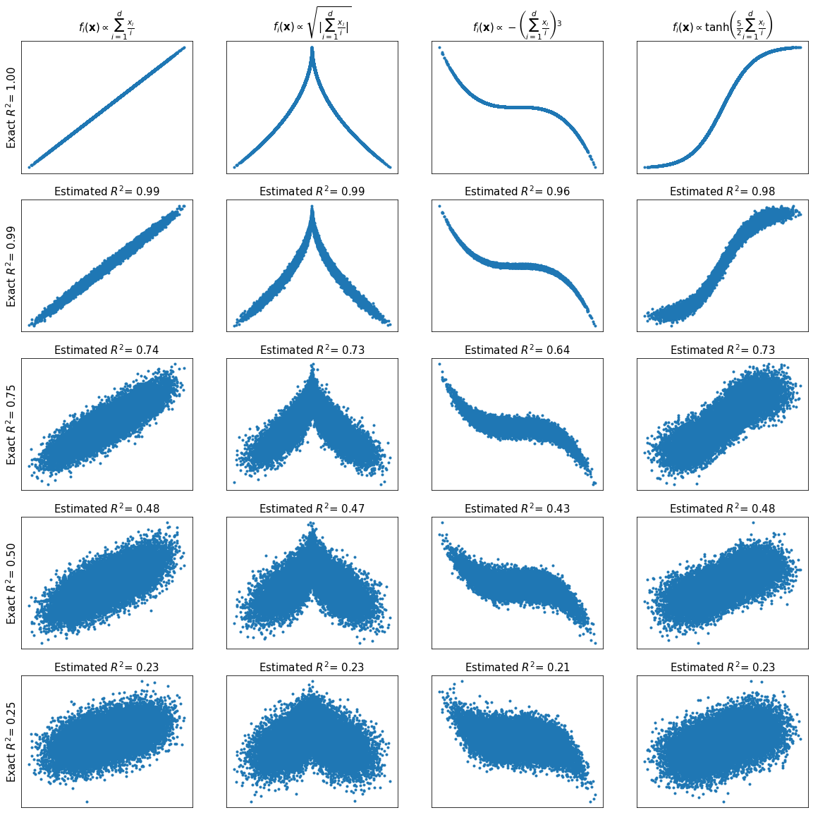
Visualizing \(R^2\) Estimation (d=10)
In [4]:
fig, axes = plt.subplots(len(rsqs), len(fs), figsize=(20, 20))
for i in range(len(rsqs)):
    for j in range(len(fs)):
        df = data[i][j].copy()
        y = df['y'].values
        axes[i, j].plot(x, y, '.')
        axes[i, j].set_xticks(())
        axes[i, j].set_yticks(())
        if i == 0:
            axes[i, j].set_title(names[j], fontsize=15)
        else:
            axes[i, j].set_title(r'''Estimated $R^2$= %.2f''' % estimated_rsqs[i][j], fontsize=15)
        if j == 0:
            axes[i, j].set_ylabel(r'''Exact $R^2$= %.2f''' % rsqs[i], fontsize=15)
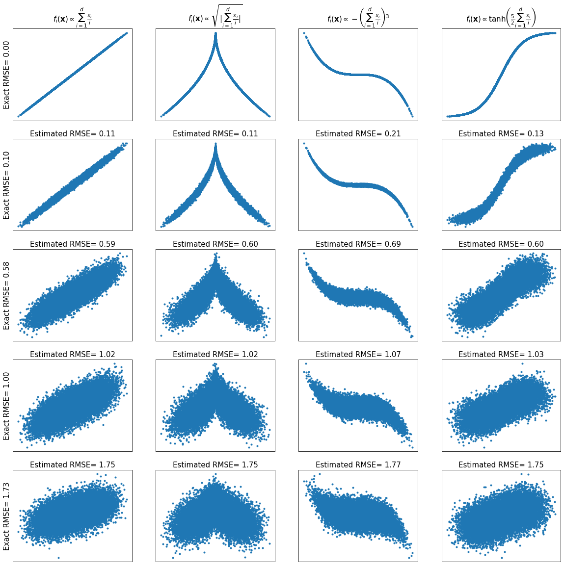
Visualizing RMSE Estimation (d=10)
In [5]:
fig, axes = plt.subplots(len(rsqs), len(fs), figsize=(20, 20))
for i in range(len(rsqs)):
    for j in range(len(fs)):
        df = data[i][j].copy()
        y = df['y'].values
        axes[i, j].plot(x, y, '.')
        axes[i, j].set_xticks(())
        axes[i, j].set_yticks(())
        if i == 0:
            axes[i, j].set_title(names[j], fontsize=15)
        else:
            axes[i, j].set_title(r'''Estimated RMSE= %.2f''' % estimated_rmses[i][j], fontsize=15)
        if j == 0:
            axes[i, j].set_ylabel(r'''Exact RMSE= %.2f''' % err_std[i], fontsize=15)